How to Unpack Dense Data in Google Sheets

There will be times when our data comes in a format that is not suitable for running summary statistics on, or really any analysis for that matter. This situation can arise when we have a column that has an array of values for each row. Ideally, we would want each of these unique values quantified somehow. Let's take a look at this so-called array-like data below:

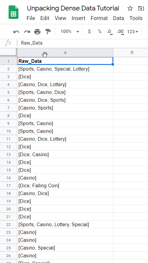
As you can see there are a handful of problems with this format. For starters, each cell has a different number of values. There are also different types of items in each list that are not necessarily present in other cells. We can resolve this through a process similar to "One Hot Encoding", or OHC for short. The idea between OHC can best be explained with a simple diagram:

The idea is to take each categorical variable and turn it into a column, and add a 1/TRUE wherever that value is present and 0/FALSE otherwise.

But do you see where our problem is?

We have multiple values in each row that need to be mapped to new columns, making our encoding process slightly more difficult. But not too difficult, don't worry! 🙂

Let's go ahead and jump in. You can access a copy of the sheet here if you wanna click around and see for yourself.

• Part 1: Parse Individual Values to New Cells
• Part 2: Get All Unique Values
• Part 3: Encode Values To Columns

PART 1: PARSE INDIVIDUAL VALUES TO NEW CELLS

This step will primarily work for cells that only contain a handful of values, otherwise the number of columns can quickly become unweildy.

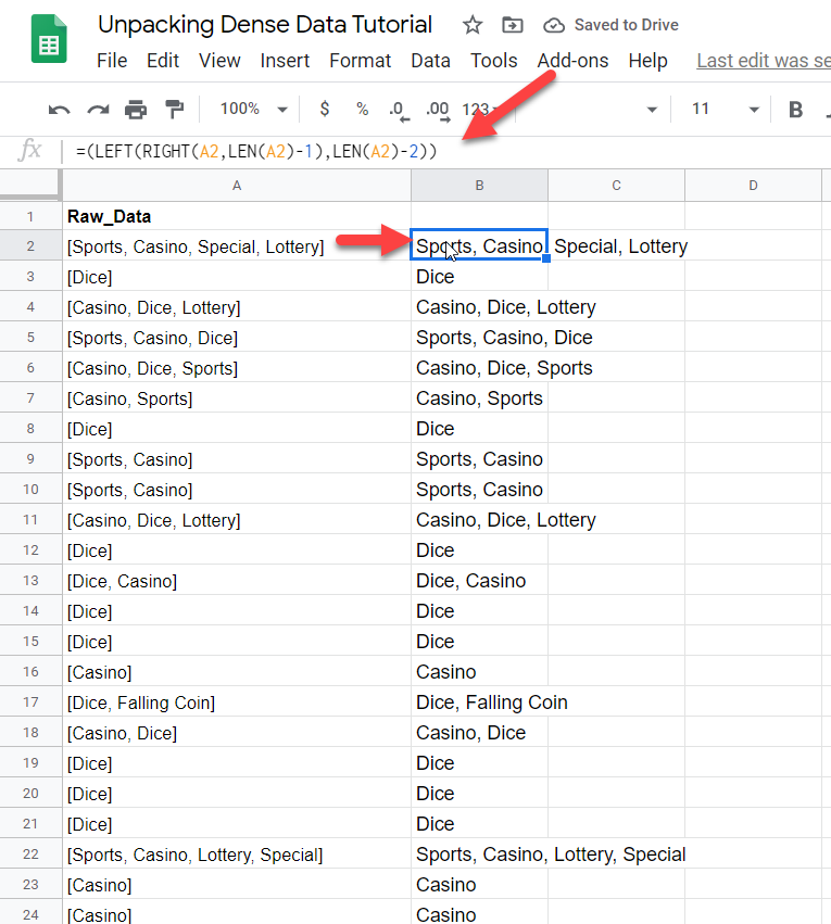
Let's head over to a new sheet, copy our raw data, and start by cleaning and parsing our cells. We can clean the brackets off the end via this formula:

=(LEFT(RIGHT(A2,LEN(A2)-1),LEN(A2)-2))

Drag it down so it gets all of the corresponding cells. At a low level, we are just removing the first and last characters (I know it's hacky, but it works!)

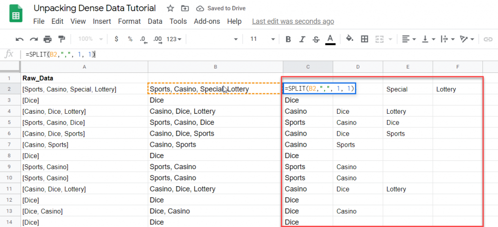
Next we need to parse out each value into a new cell. We can accomplish this by spiting along commas with the following formula:

=ARRAYFORMULA(TRIM(SPLIT(B2,",", 1, 1)))

PART 2: GET ALL UNIQUE VALUES

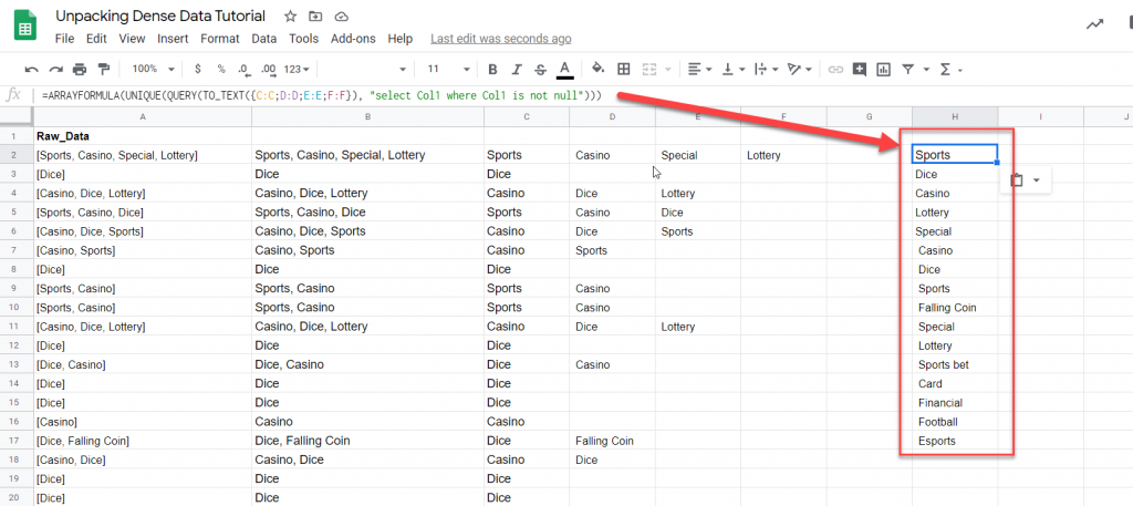
Sheets has a UNIQUE() function that is great for individual columns. But what if we want to get all unique values across multiple columns? We gotta break out some serious fire power for this scenario unfortunately. In a nut shell, we will need to "stack" our columns on top of each other via the semi-colon and curly brackets syntax, i.e. {A:A;B:B}, followed by a Sheets QUERY() function to filter out any null values, followed by the UNIQUE() function to get any unique values from our fake column, then lastly ARRAYFORMULA() to make it work for multiple source columns. So with all the theory aside, the formula looks like this:

=ARRAYFORMULA(UNIQUE(QUERY(TO_TEXT({C:C;D:D;E:E;F:F}), "select Col1 where Col1 is not null")))

And you should end up with this:

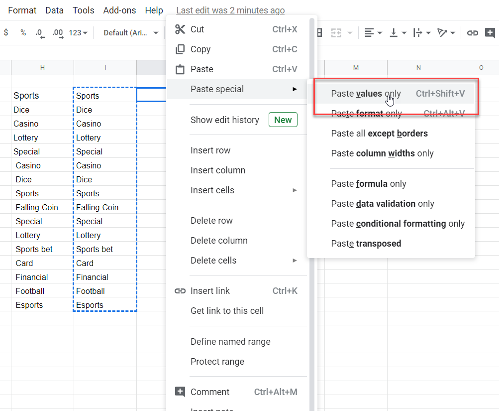
And lastly, copy and special paste the last column as values only:

PART 3: ENCODE VALUES TO COLUMNS

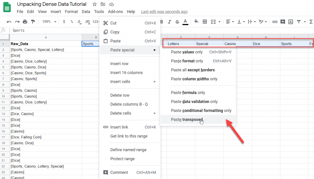
Now for the fun part! We need to take these unique value names, create new columns back in our original datasheet, and then reference the dense rows to mark our columns as either True or False (or 1 / 0). To start, we will need to copy and paste special transpose our unique values like below:

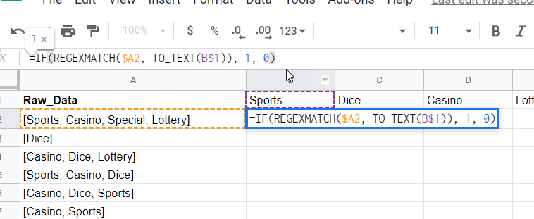
Now, we need to setup an IF statement with a Regular Expression to accomplish this. We will reference the column's name and check if the dense cell contains a value corresponding to the column name. The formula looks like this:

=IF(REGEXMATCH($A2, TO_TEXT(B$1)), 1, 0)

Now that we have this, drag our cell down and across to make what is known as a "sparse matrix".

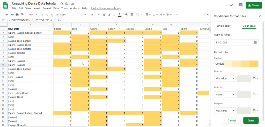
Congratulations! You have successfully unpacked and encoded your data into columns!